Intro
Welcome folks, I hope you are keeping safe and well. I’m going to spend some time on a series of articles and some tooling to aid in the creation of brushes and technical art for TiltBrush software.
This article is intended to be the first in a series. Please be aware that the Python code in this article and in the associated toolset is deliberately written to be verbose and expressive. I have taken this approach because I want it to be accessible and easily understood. This is not optimal python, nor good style. You have been warned!
Well, without further ado lets jump right in.
Stroke And Line Primitive
The most fundamental aspect of a TiltBrush sketch is called a Control Point.
This is essentially a single vertice on a curve in 3-dimensional space with
a couple of other properties, such as pressure and timestamp. These properties
combined are used when rendering a brush stroke. For this project we will first
need to build a line primitive, which we will later use to build other more
complex primitives.
(If you would like to read more information about the TiltBrush file format, I have written about it before here).
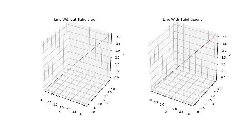
Creating A Line Primitive And Subdivision
A stroke in a TiltBrush sketch is a series of ordered Control Points.
We can represent this stroke as a 3 dimensional line in our code. We will
need to make sure that the vertices on the line are equidistant, not spaced too
far apart, and in the correct order with no duplicates.
This is easy enough to achieve with a recursive function that finds the midpoint of a line segment until the line segment length is short enough and then exits up through the recursion. As a refresher, the midpoint and segment length formulas in 2d and 3d are.
Segment Length
2D
$$ d = \sqrt{(x2 -x1)^2 + (y2 - y1)^2} $$3D
$$ d = \sqrt{(x2 -x1)^2 + (y2 - y1)^2 + (z2 - z1)^2} $$Midpoint
2D
$$ (x,y) = \left(\dfrac{x1+x2}2,\dfrac{y1+y2}2\right) $$3D
$$ (x,y,z) = \left(\dfrac{x1+x2}2,\dfrac{y1+y2}2,\dfrac{z1+z2}2\right) $$Most of the code to solve this is mundane, but I did like the recursive method of subdividing the line segments. When I am finished this experimental project and series of blog articles I’ll share all of the code and tools with you.
    def __subdivide(self, segment):
        seg_len = self.__length(segment)
        if seg_len < self.max_seg_size:
            self.ctrl_pts.append(segment)
            return

        segments = self.__split_segment(segment)
        for s in segments:
            self.__subdivide(s)
Once these operations are complete we have a nice subdivided line segment which can be used to render a stroke inside of TiltBrush.
A Quick Digression About Centroids
Although it is not necessary I think it is very convenient to have polyhedra transformations based on the centroid or center mass of the polyhedra. This makes it much easier to postion shapes based on world coordinates.
It took a while to find good solutions that derive the centroid of polyhedra. I found two recommended solutions, both apply to non-self-intersecting closed 3D polyhedron but obtain two different properties. I’m going to stand on the shoulders of giants, and convert these solutions to code.
The first approach uses an average of the vertice vectors in a mesh to obtain the centroid of the vertices – the second uses a divergence theorem to obtain the center-mass (and area) of the polyhedra. Both properties are very useful for different types of meshes (3d line vs 3d mesh for example)
To aid in computing the above I created a vector class for 3 dimensions, and added some utility methods to it for calculating dot, and cross products – as well as magnitude and direction. I also added some functionality to facilitate vector arithmetic. This class can be found in the reference section of this article.
Lets sketch some utility code to calculate centroids.
Centroid Of Vertices
The centroid of the vertices is the point derived from the arithmetic mean of all of the vertices in the polyhedra. This is the case for 2, 3, and indeed n-dimensions.

To obtain the centroid of a list of vertices , first organize the vertice point data as follows:
$$ P = \begin{bmatrix} x_1 & x_2 & x_3 & \dots &x_n\\ y_1 & y_2 & y_3 & \dots &y_n\\ z_1 & z_2 & z_3 & \dots &z_n\\ \end{bmatrix} $$In our code, this is a pretty simple operation, but it makes the centroid calculation easier in the next step.
    rows = 3        # x, y, z
    cols = len(PTS) # n
    P = zeros_matrix(rows, cols)
    # populate the matrix
    for i in range(rows):
        for j in range(cols):
            P[i][j] = PTS[j][i]
And now to calculate the centroid C, we just iterate over the matrix P and
obtain the arithmetic average.
Which translates to the following python code.
    lst = []
    for i in range(cols):
        _m = zeros_matrix(1, 3)
        _m[0][0] = P[0][i]
        _m[0][1] = P[1][i]
        _m[0][2] = P[2][i]
        lst.append(_m)

    _msum = add_matrices(lst)
    sc = 1 / cols
    centroid_matrix = multiply_matrix_by_scalar(_msum, sc)
And that is it!
Centroid Of Triangles
Calculating the centroid using the triangles (faces) of a polyhedra is more involved. Actually, surprisingly more involved. It requires some intricate (for me) calculus for a general solution.
It took me a long time to understand this approach as my calculus is rusty. To be frank I still do not have a firm intuition for this. I will try to revisit this in a future article as it is extremely interesting to me. I do understand it from the application perspective so I am going to forge forward. Just be comforted, that if you find this math difficult to grok, you are not alone.
The process is described precisely here, I will include the formula and my translation of it to python code.
In this approach Ai (i=0 -> N-1) is the count of triangular faces on the polyhedron P.
So Ai is a triangle. For each of these triangles i– it is assumed that the vertices of the
triangle ai, bi, ci are ordered counter clockwise. We can calculate the outer unit-normal
n for each triangle of P as.
The little ^ symbol means unit vector, the ⊗ is the product measure. From this, we can
calculate the volume V of P using the divergence theorem
this is because x · nᵢ is a constant on each triangle and the area of each triangle is:
$$\cfrac{1}{2}|\hat{n_i}|$$
The theorem has the following form, the sigma is sort of like a for loop. The long S type symbol is a definite integral which can be thought of as a sort of sum function – these functions are used a lot in calculus to derive areas – specifically areas under curves. There is a good intro to integral calculus here
$$ V = \int_{P}\enspace 1 = \cfrac{1}{3}\int_{\partial P}\enspace x \cdot n = \cfrac{1}{3}\sum_{i=0}^{N-1}\int_{A_i} \enspace a_i \cdot n_i = \cfrac{1}{6}\sum_{i=0}^{N-1}a_i\cdot \hat{n_i} $$So the centroid of P will be in set of real numbers in 3 dimensions R3. Where C is centroid,
and V is volume:
We now apply the divergence theorem again, where the standard basis is denoted as e1, e2, e3, allowing us to obtain the three coordinates of the centroid:
This expands to this rather unaproachable system, which can be converted to python code.
$$ \int_{A_i} (x \cdot e_d)^2(n_i \cdot e_d) \\\\ = \frac{1}{6} \hat{n_i} \cdot e_d([\frac{1}{2}(a_i+b_i)\cdot e_d]^2 + [\frac{1}{2}(b_i+c_i)\cdot e_d]^2 + [\frac{1}{2}(c_i+a_i)\cdot e_d]^2)\\\\ = \frac{1}{24} \hat{n_i} \cdot e_d([(a_i + b_i) \cdot e_d]^2 + [(b_i + c_i) \cdot e_d]^2 + [(c_i + a_i) \cdot e_d]^2) $$I do not fully understand how the above relates to the standard midpoint sampling quadrature formula for triangles, that remains to be explored.
This is the translation to code, triangle is a custom class that I created to represent a
triangle – properties a, b, and c are vector3 objects – remember my vector3 class
is in the reference section). triangles is an ordered list of triangle objects obtained from
parsing a mesh.
    total_volume = 0.0
    centroid_integral = Vec3.zero()

    # for each triangle in an ordered list of triangles that make up the mesh
    for triangle in triangles:
        b_a = triangle.b - triangle.a
        c_a = triangle.c - triangle.a

        # compute area-magnitude normal for this triangle and add it to the
        # total volume of this polyhedra
        n = b_a.cross(c_a)
        total_volume += triangle.a.dot(n) / 6.0

        # compute and then add the current triangle contribution to the overall
        # centroid integral for each dimension.

        # X
        x_contribution = n.x * math.pow((triangle.a.x + triangle.b.x), 2) +
                               math.pow((triangle.b.x + triangle.c.x), 2) +
                               math.pow((triangle.c.x + triangle.a.x), 2)
        centroid_integral.x = centroid_integral.x + x_contribution

        # Y
        y_contribution = n.y * math.pow((triangle.a.y + triangle.b.y), 2) +
                               math.pow((triangle.b.y + triangle.c.y), 2) +
                               math.pow((triangle.c.y + triangle.a.y), 2)
        centroid_integral.y = centroid_integral.y + y_contribution

        # Z
        z_contribution = n.z * math.pow((triangle.a.z + triangle.b.z), 2) +
                               math.pow((triangle.b.z + triangle.c.z), 2) +
                               math.pow((triangle.c.z + triangle.a.z), 2)
        centroid_integral.z = centroid_integral.z + z_contribution

    # finally scale each centroid dimension by the inverse volume
    x_scaled = centroid_integral.x * (1.0 / (24.0 * 2.0 * total_volume))
    y_scaled = centroid_integral.y * (1.0 / (24.0 * 2.0 * total_volume))
    z_scaled = centroid_integral.z * (1.0 / (24.0 * 2.0 * total_volume))

    # and return the centroid!
    return Vec3(x_scaled, y_scaled, z_scaled)
Code / Implementation Test
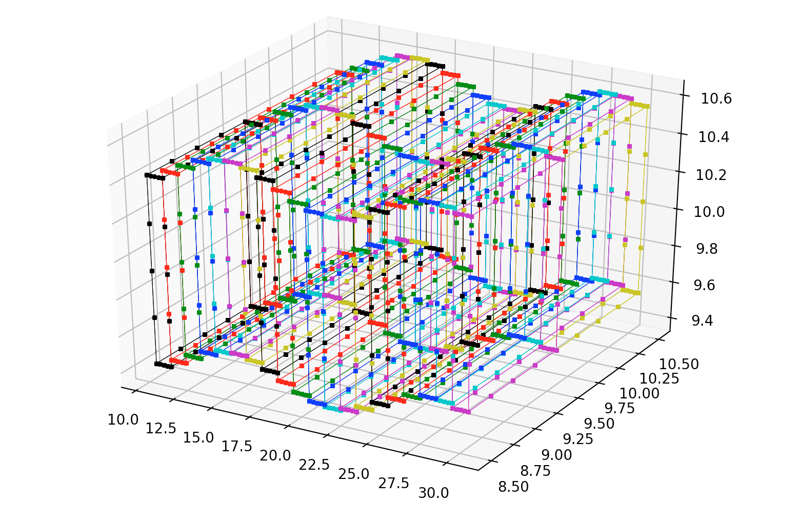
We can now apply the above theory and code to derive the centroid of a mesh. I found a mesh pumpkin online which is a pretty nice test. It is low-poly, and it has an unusual shape. It is also an enclosed polyhedra that does not self-intersect. Here are the results, the red point is the centroid.
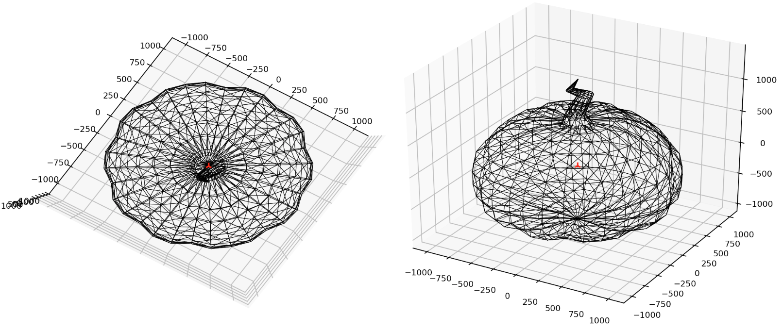
That was fun! I didn’t anticipate this complexity, so it turned into a really neat little adventure. Now lets move onwards! Lets get this picture printed!
Rotation And Translation
To generate art using our work above, we will need to create some shape primitives. But before we do that, we also need to know how to rotate, and position these primitives otherwise it would be a very boring picture consisting of all pixels overlapped in a single position 😂
In the future we will discuss and add functionality to scale, and also skew primitives too!
Translation
The translation operation should displace all of the points in a geometric object by a fixed distance in a given direction. The formula for a translation is:
$$ P' = P + d $$For all points P on the object. This translates (🥁) to the following python code.
We use our vertice centroid solution that we discussed earlier.
def translate_by_centroid3d(centroid, delta, vertices):
    # translate centroid
    translated_centroid = translate_vertice3d(centroid, delta)

    dv = (translated_centroid[0] - centroid[0],
          translated_centroid[1] - centroid[1],
          translated_centroid[2] - centroid[2])

    translated_vertices = []
    for v in vertices:
        x = v[0]
        y = v[1]
        z = v[2]
        tx = x + dv[0]
        ty = y + dv[1]
        tz = z + dv[2]
        translated_vertices.append((tx, ty, tz))

    return (translated_centroid, translated_vertices)

def translate_vertice3d(vertice, delta):
        x = vertice[0]
        y = vertice[1]
        z = vertice[2]
        tx = x + delta[0]
        ty = y + delta[1]
        tz = z + delta[2]

        return (tx, ty, tz)
Rotation
A rotation operation is a little more involved, we want to rotate a 3d shape around its centroid. The transformation matrix for this operation is:
$$ Rx = Rx(\theta) = \begin{bmatrix} 1 & 0 & 0 \\ 0 & \cos\theta & -\sin\theta \\ 0 & \sin\theta & \cos\theta \end{bmatrix} \\\\ \enspace \\\\ Ry = Ry(\theta) = \begin{bmatrix} \cos\theta & 0 & \sin\theta \\ 0 & 1 & 0 \\ -\sin\theta & 0 & \cos\theta \end{bmatrix} \\\\ \enspace \\\\ Rz = Rz(\theta) = \begin{bmatrix} \cos\theta & -\sin\theta & 0 \\ \sin\theta & \cos\theta & 0 \\ 0 & 0 & 1 \end{bmatrix} $$We can create the following code that mostly emulates the above transformation. But we will approach scale and skew in another post. For now, this is my naive solution:
def rotate3d(angle, vertices):
    rvertices = rotate_x(angle[0],vertices)
    rvertices = rotate_y(angle[1],rvertices)
    rvertices = rotate_z(angle[2],rvertices)

    return rvertices

def rotate_x(theta, vertices):
    sin_theta = math.sin(theta)
    cos_theta = math.cos(theta)

    rotated_vertices = []
    for v in vertices:
        print(":",v)
        x = v[0]
        y = v[1]
        z = v[2]
        rx = x
        ry = y * cos_theta - z * sin_theta
        rz = z * cos_theta + y * sin_theta
        rotated_vertices.append((rx, ry, rz))

    return rotated_vertices

def rotate_y(theta, vertices):
    sin_theta = math.sin(theta)
    cos_theta = math.cos(theta)

    rotated_vertices = []
    for v in vertices:
        x = v[0]
        y = v[1]
        z = v[2]

        rx = x * cos_theta + z * sin_theta
        ry = y
        rz = z * cos_theta - x * sin_theta
        rotated_vertices.append((rx, ry, rz))

    return rotated_vertices

def rotate_z(theta, vertices):
    sin_theta = math.sin(theta)
    cos_theta = math.cos(theta)

    rotated_vertices = []
    for v in vertices:
        x = v[0]
        y = v[1]
        z = v[2]

        rx = x * cos_theta - y * sin_theta
        ry = y * cos_theta + x * sin_theta
        rz = z
        rotated_vertices.append((rx, ry, rz))

    return rotated_vertices
Pixels And Voxels!
To make this article a reasonable size, we will focus on a two simple primitives first then in future articles we will get more advanced. For now we will make pixels and voxels! I think we all know what pixels are, but a voxel is a cuboid, its a pixel for 3-dimensions.
Pixels
I created a pixel as a square that consisted of four lines in Tiltbrush, and then two
lines that form an X as the fill for the pixel. I have included the code below:
class TBPixel:
    """
        This class represents a pixel in a tiltbrush drawing. It
        contains an array of strokes used to draw the cuboid.

              3-------2
              |       |
              |       |
              |       |
              0-------1
    """
    def __init__(self, position, color, width, height):  # w, h
        assert_valid_vec3_type(position)
        assert_valid_float_type(width)
        assert_valid_float_type(height)
        assert_valid_tb_color_type(color)

        self.__plane = Plane(position, width, height)
        self.__color = color
        self.__strokes_filled = ()
        self.__strokes_unfilled = ()
        self.__generate_strokes()

    @property
    def position(self):
        return self.__plane.position

    @position.setter
    def position(self, position):
        assert_valid_vec3_type(position)
        self.__plane.position = position
        self.__generate_strokes()

    @property
    def strokes_filled(self):
        return self.__strokes_filled

    @property
    def strokes_unfilled(self):
        return self.__strokes_unfilled

    @property
    def color(self):
        return self.__color

    @property
    def plane(self):
        return self.__plane

    def __generate_strokes(self):
        # line from 0 -> 1
        s0 = TBLine(self.plane.pt0, self.plane.pt1)

        # line from 1 -> 2
        s1 = TBLine(self.plane.pt1, self.plane.pt2)

        # line from 2 -> 3
        s2 = TBLine(self.plane.pt2, self.plane.pt3)

        # line from 3 -> 0
        s3 = TBLine(self.plane.pt3, self.plane.pt0)

        self.__strokes_unfilled = (s0, s1, s2, s3)

        # now make the X in the middle
        # line from 0 -> 2
        sx1 = TBLine(self.plane.pt0, self.plane.pt2)

        # line from 1 -> 3
        sx2 = TBLine(self.plane.pt1, self.plane.pt3)

        self.__strokes_filled = (s0, s1, s2, s3, sx1, sx2)
Voxels
For the voxels, the approach is similar to the pixel above, only we create 6 faces (6 pixels) that make up a cube shape. I have included the code below:
class TBCuboid:
    """
        This class represents a cuboid in a tiltbrush drawing. It
        contains an array of strokes used to draw the cuboid.

                7-------6 (max)
               /|      /|
              4-+-----5 |
              | |     | |   y (+)
              | 3-----+-2   |
              |/      |/    |/
        (min) 0-------1   --+-----x (+)
                           /
                          z (+)

        Front-Back or Back-Front Z-Axis
    """
    def __init__(self, position, color, size=Vec3(1.0, 1.0, 1.0)):  # w, h, d
        assert_valid_vec3_type(position)
        assert_valid_vec3_type(size)
        assert_valid_tb_color_type(color)

        self.__cuboid = Cuboid(position, size)
        self.__color = color
        self.__generate_strokes_unfilled()

    @property
    def faces(self):
        return (self.__face1, self.__face2, self.__face3, self.__face4, self.__face5, self.__face6)

    @property
    def color(self):
        return self.__color

    @property
    def cuboid(self):
        return self.__cuboid

    def __generate_strokes_unfilled(self):

        # left face stroke
        lf_sl_0_3 = TBLine(self.cuboid.pt0, self.cuboid.pt3)
        lf_sl_3_7 = TBLine(self.cuboid.pt3, self.cuboid.pt7)
        lf_sl_7_4 = TBLine(self.cuboid.pt7, self.cuboid.pt4)
        lf_sl_4_0 = TBLine(self.cuboid.pt4, self.cuboid.pt0)
        self.__face1 = TBFace(lf_sl_0_3, lf_sl_3_7, lf_sl_7_4, lf_sl_4_0)

        # back face stroke
        bf_sl_3_2 = TBLine(self.cuboid.pt3, self.cuboid.pt2)
        bf_sl_2_6 = TBLine(self.cuboid.pt2, self.cuboid.pt6)
        bf_sl_6_7 = TBLine(self.cuboid.pt6, self.cuboid.pt7)
        bf_sl_7_3 = TBLine(self.cuboid.pt7, self.cuboid.pt3)
        self.__face2 = TBFace(bf_sl_3_2, bf_sl_2_6, bf_sl_6_7, bf_sl_7_3)

        # right face stroke
        rf_sl_1_2 = TBLine(self.cuboid.pt1, self.cuboid.pt2)
        rf_sl_2_6 = TBLine(self.cuboid.pt2, self.cuboid.pt6)
        rf_sl_6_5 = TBLine(self.cuboid.pt6, self.cuboid.pt5)
        rf_sl_5_1 = TBLine(self.cuboid.pt5, self.cuboid.pt1)
        self.__face3 = TBFace(rf_sl_1_2, rf_sl_2_6, rf_sl_6_5, rf_sl_5_1)

        # front face stroke
        ff_sl_0_1 = TBLine(self.cuboid.pt0, self.cuboid.pt1)
        ff_sl_1_5 = TBLine(self.cuboid.pt1, self.cuboid.pt5)
        ff_sl_5_4 = TBLine(self.cuboid.pt5, self.cuboid.pt4)
        ff_sl_4_0 = TBLine(self.cuboid.pt4, self.cuboid.pt0)
        self.__face4 = TBFace(ff_sl_0_1, ff_sl_1_5, ff_sl_5_4, ff_sl_4_0)

        # top face stroke
        tf_sl_4_5 = TBLine(self.cuboid.pt4, self.cuboid.pt5)
        tf_sl_5_6 = TBLine(self.cuboid.pt5, self.cuboid.pt6)
        tf_sl_6_7 = TBLine(self.cuboid.pt6, self.cuboid.pt7)
        tf_sl_7_4 = TBLine(self.cuboid.pt7, self.cuboid.pt4)
        self.__face5 = TBFace(tf_sl_4_5, tf_sl_5_6, tf_sl_6_7, tf_sl_7_4)

        # bottom face stroke
        bf_sl_0_1 = TBLine(self.cuboid.pt0, self.cuboid.pt1)
        bf_sl_1_2 = TBLine(self.cuboid.pt1, self.cuboid.pt2)
        bf_sl_2_3 = TBLine(self.cuboid.pt2, self.cuboid.pt3)
        bf_sl_3_0 = TBLine(self.cuboid.pt3, self.cuboid.pt0)
        self.__face6 = TBFace(bf_sl_0_1, bf_sl_1_2, bf_sl_2_3, bf_sl_3_0)
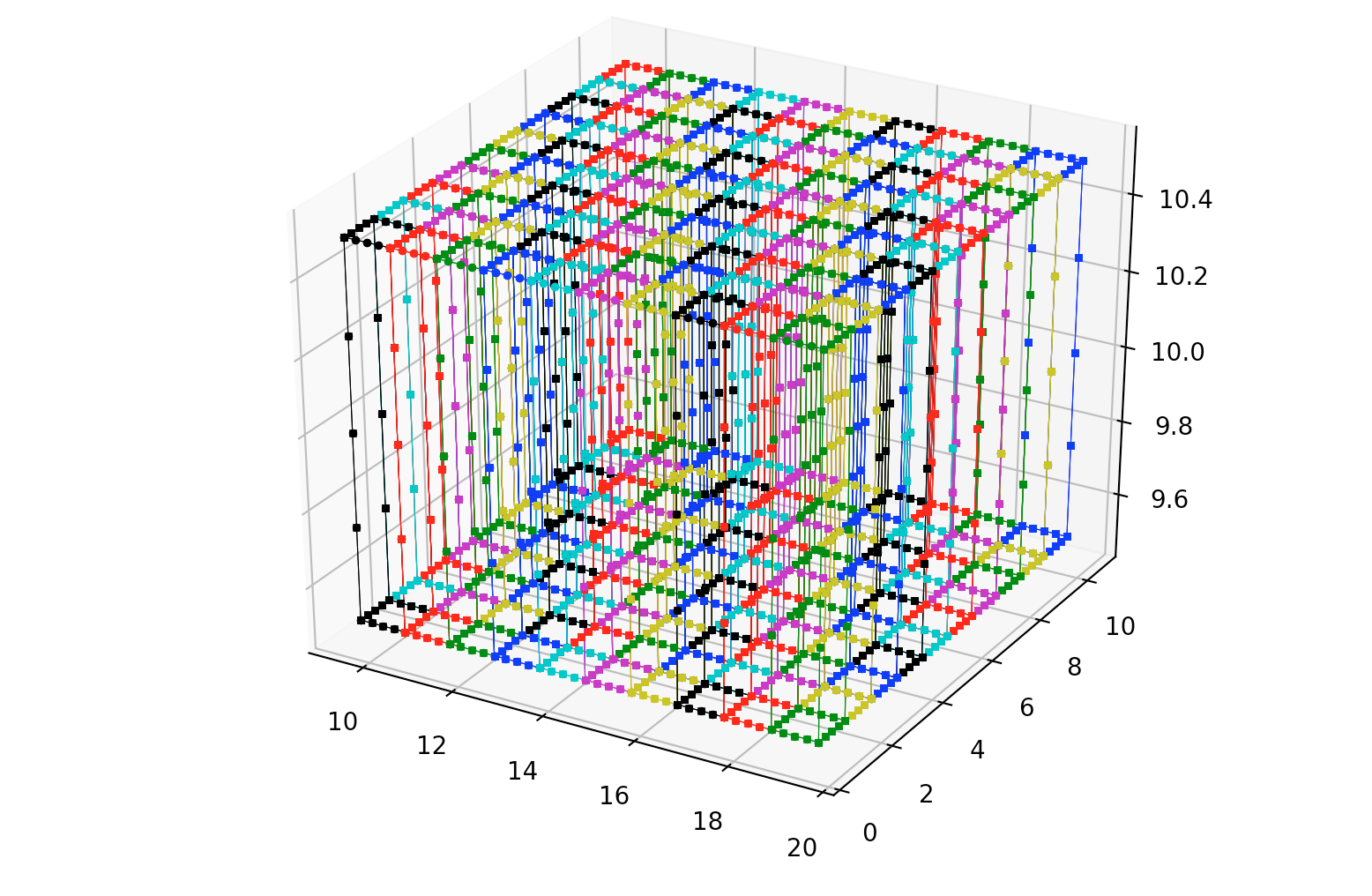
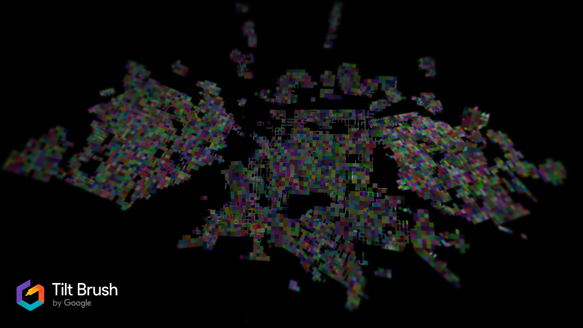
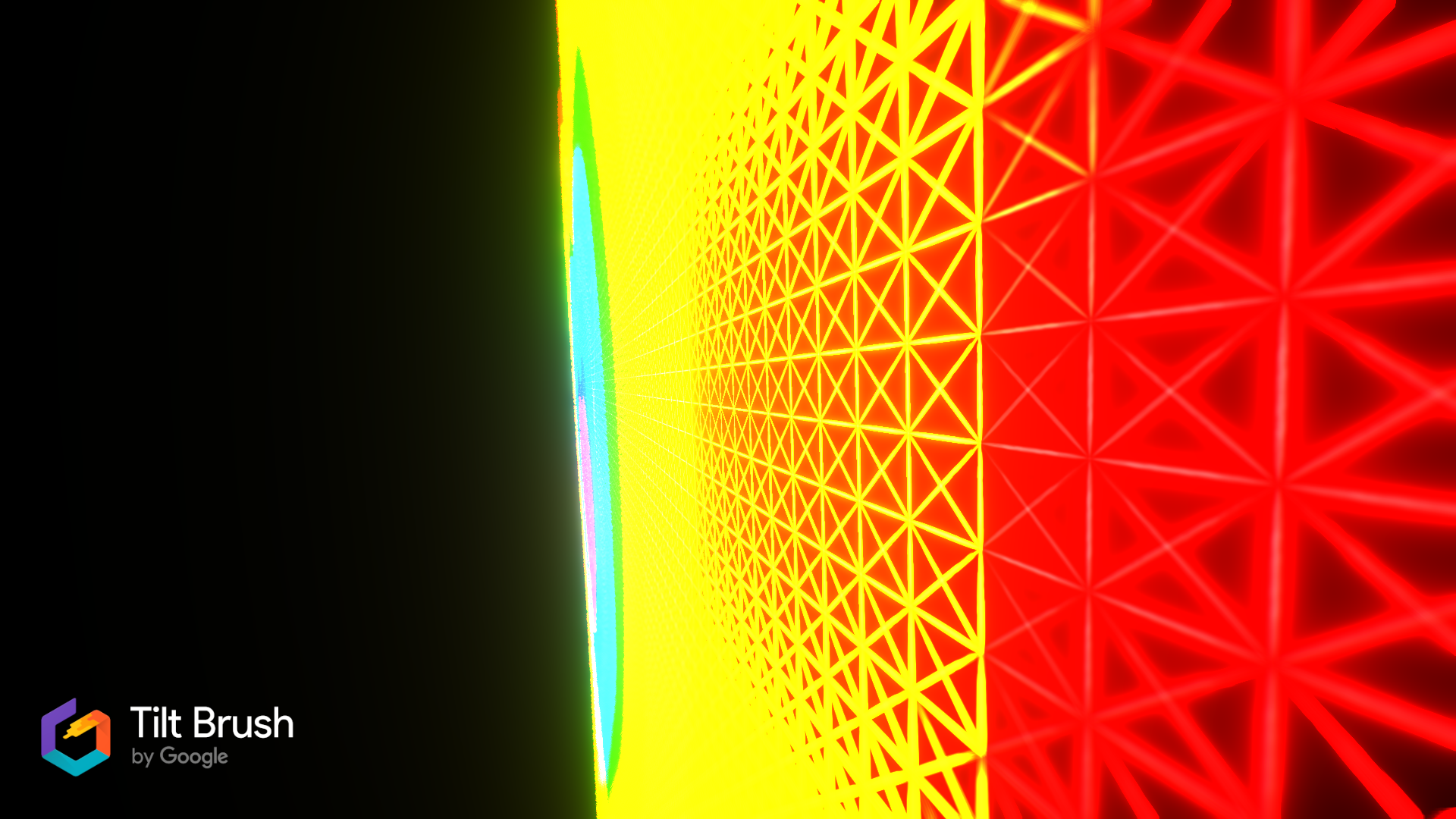
By combining all of the above its possible to render voxels into a Tiltbrush painting, as can be seen in the figure below (left) [lit hull brush]. By playing with the color and translation, its possible to build a giant wall of voxels ୧⍢⃝୨, as can be seen on the figure below (right).
We can massage this structure inside TiltBrush and use it as a base for other art. We will revisit this in the future, but the idea is to create primitive brushes that can be used for other paintings!
Surface Deformations
We could print out picture in VR as a flat image, but I wanted to make it a little more interesting. If we pass the position through a sine function we can make it have a nice wave effect on the print.
I hope this gives a taste of what can be done with positions and rotations in the future! Now we have the tools we need to print a picture so lets march forward!!
Bitmaps And PNGs
So next we need to process a source image so that we can print it into virtual reality 👩🏼🎤. When I was thinking about this article initially I thought that it would be a good idea to use the bitmap file format. If you are unaware, bitmap files are quite easy to parse once they are not compressed.
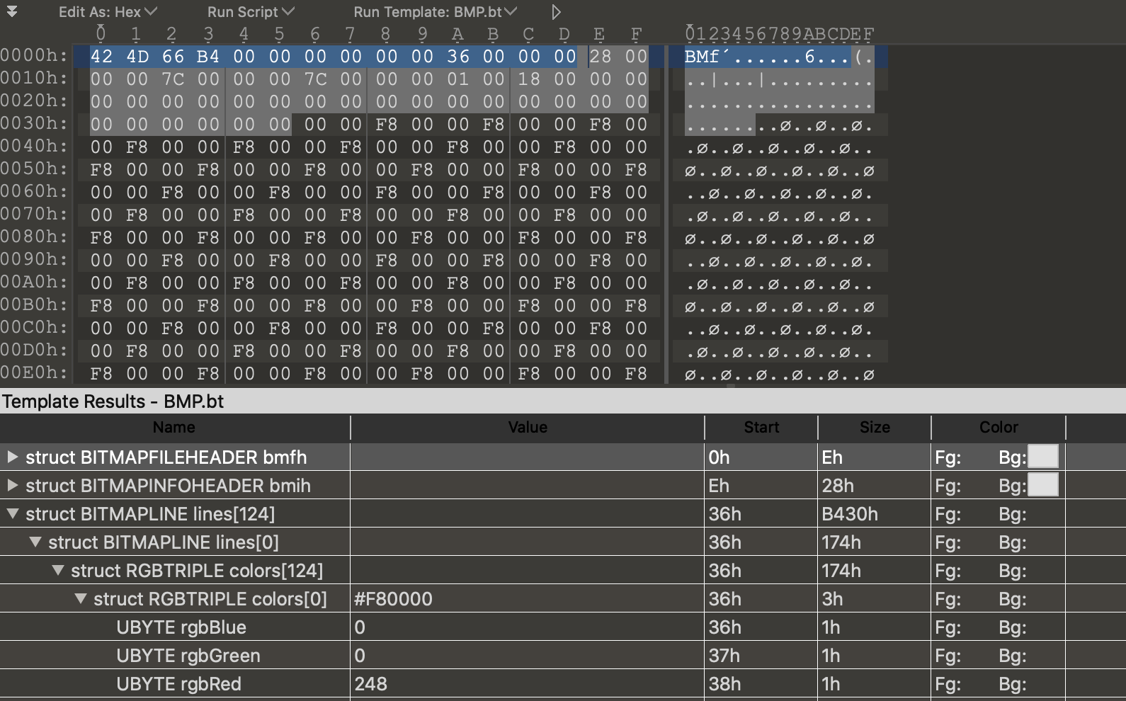
A bitmap file consists of a file header, an info header, and then a series of bytes representing the Red Green and Blue colors (RGB). However, after some thought I decided that this file format is kind of archaeic and not very common online. It also doesn’t support an alpha (transparency) channel which I find essential. I really don’t want people to need to convert the image file to a different file format before printing it. For this reason I began examining PNG image files instead.
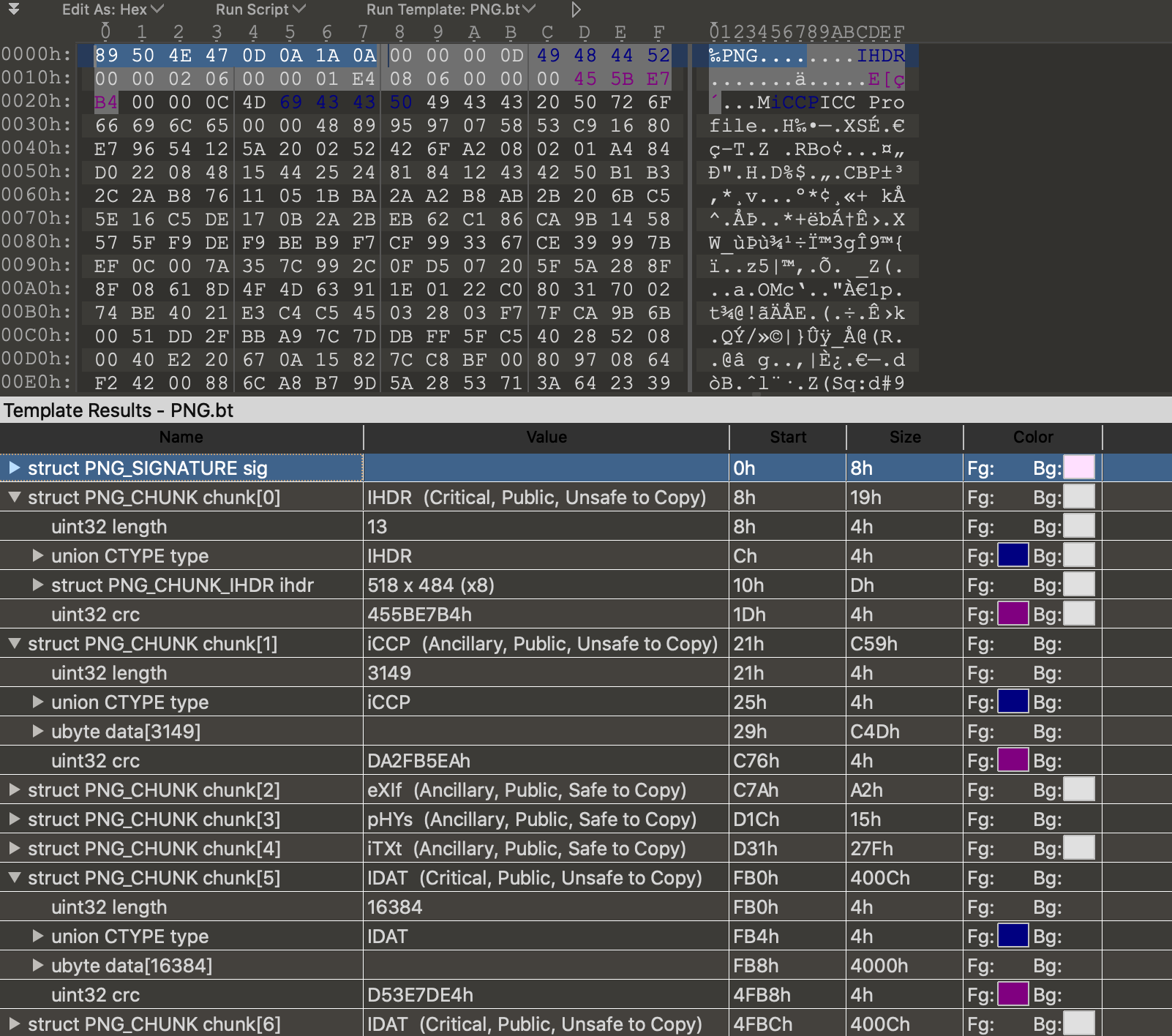
The PNG file structure is definitely more complicated than a Bitmap file. The file starts with a PNG file header:
OFFSET              Count TYPE   Description
0000h                   8 char   ID=89h,'PNG',13,10,26,10
But the rest is a series of chunks which consist of chunk length, a type, data,
and a cyclical redundency checksum (crc). I began writing a parser from scratch
but I think it is outside the scope of the time I allocated to this project so
instead I installed PIL and it made loading a PNG image very easy:
    def __load_file(self, f):

        if not path.exists(f):
            raise FileNotFoundError("File doesn't exist!")
        else:
            im = Image.open(f, 'r')
            self.size = im.size
            self.mode = im.mode
            self.width, self.height = im.size
            self.rows = self.height
            self.cols = self.width

            _pixels = list(im.getdata())
            self.pixels = \
              [_pixels[i * self.width:(i + 1) * self.width] for i in range(self.height)]
            self.initialized = True
We expand on this a little and make a class to hold each pixel as a custom color type. This will allow us to process the pixels easier when rendering into TiltBrush.
class TBColor:
    def __init__(self, color=Vec3(0.0, 0.0, 0.0), alpha=1.0, transparency_threshold=0.1):

        if color.x > 1.0 or color.y > 1.0 or color.z > 1.0:
            raise("Color range is 0.0 -> 1.0")

        if color.x < 0.0 or color.y < 0.0 or color.z < 0.0:
            raise("Color range is 0.0 -> 1.0")

        self.__red = color.x
        self.__green = color.y
        self.__blue = color.z
        self.__alpha = alpha
        self.__transparency_threshold = transparency_threshold
        self.__is_transparent = (True if (self.__alpha < self.__transparency_threshold) else False)

    @staticmethod
    def random():
        return TBColor(Vec3(random(), random(), random()))

    @property
    def r(self):
        return self.__red

    @property
    def g(self):
        return self.__green

    @property
    def b(self):
        return self.__blue

    @property
    def is_transparent(self):
        return self.__is_transparent

    @property
    def a(self):
        return self.__alpha

    @property
    def rgb(self):
        return (self.r, self.g, self.b)

    @property
    def rgba(self):
        return (self.r, self.g, self.b, 1.0) # I don't think alpha works in TiltBrush
Pixel Print
So the next thing we need to do is scan an image into a pixel array, and then plot this image using all of the work we have done above.
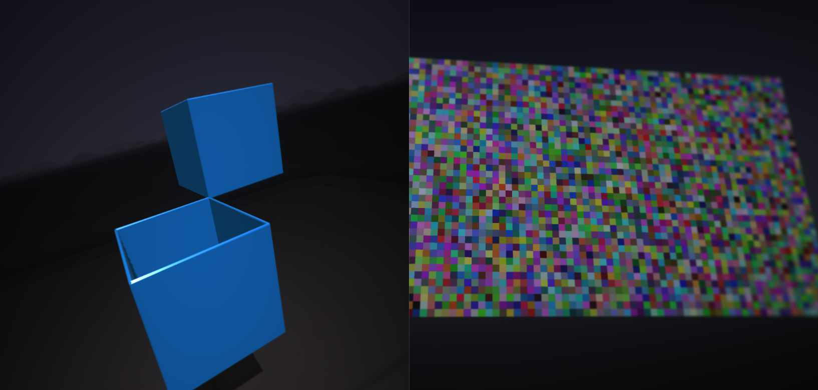
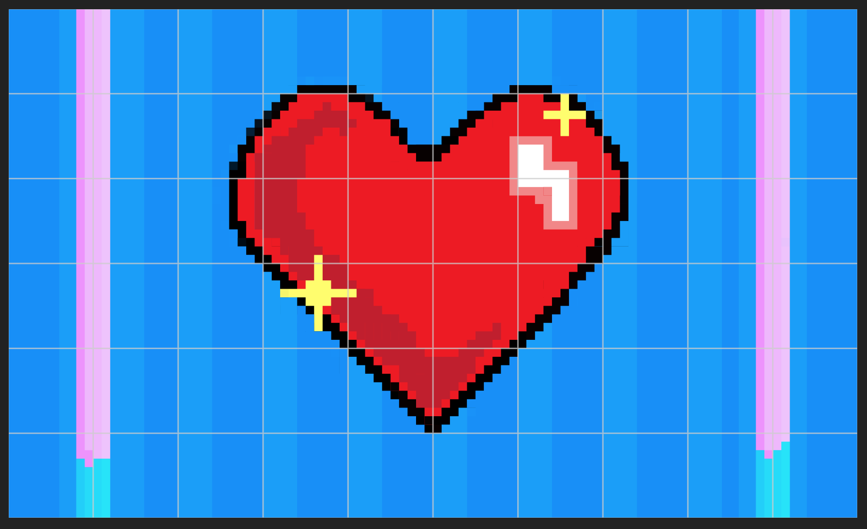
I found the following image online, it is Creative Commons so I figured it would be ok to use it as an example. Its got a really nice color range! Who doesn’t like rainbows? Its got an alpha channel too which was interesting to process.

I loaded the image using our work above, and printed it into a TiltBrush painting. Each pixel
is filled using 2 diagonal lines. This is the X pattern on each pixel that we discussed
earlier, it can be seen in the closeup screenshots below.
![]()
The code to create the pixels is pretty nice at this point, as a lot of the details are
neatly abstracted. It could certainly be improved on though. We can also skip the pixels
that are transparent using the color.is_transparent predicate below.
for row in range(0, ROWS):
    print("row %d of %d rows" % (row, ROWS))
    for col in range(0, COLS):
        position.x += pixel_width
        color = tb_img.pixel_at(row, col)
        # don't create a pixel if it is transparent
        if color.is_transparent:
            continue

        pixel = TBPixel(position, color, pixel_width, pixel_height)
        pixels.append(pixel)

    position.y -= pixel_height
    position.x = start_position.x
And there we have it, a PNG scanned and printed into VR using Tiltbrush brush-strokes. The image took a while to load, and this is what it looks like in VR!

Note that the bloom on the shader makes the colors wash out and bleed into each other a little, especially the brighter colors like Yellow and Cyan 😄. This is pretty interesting and might make a good topic for a different blog article – I still think it looks neat ! Also its nice that there is room for improvement.
Its also difficult to communicate the size of this heart as it appears in VR, it feels like it is 50 meters tall 😂.
Voxel Print
So next we are going to print a picture using our work on voxel printing above. In this case I made a tiny flag (ratio 3:5) using pixel art. The flag is 100 x 60 pixels.
At the moment it is very important to consider the pixel count in the image, because we have not optimized the voxel renderer at all – and so it prints hidden faces and doesnt merge visible faces. This means that it is not performant at all, for example the image above will produce approximately 36,000 planes/faces. This in turn will have even more faces rendered by the surface shader that Tiltbrush applies to the brush that we have chosen (lit hull brush.)
The flag source image is tiny :

And here it is rendered into a massive Tiltbrush picture with a sine applied to shape the z-axis position of each voxel. It translates pretty well hey? I love how accurate the colors are!


I’m dissapointed that I ran out of time allocated to this article, but the curvature of the flag wave could be drastically improved. Lets revisit this in the future. I still think it looks pretty neat.
Et Voila
Putting all of the above together and we have some tools to print images into Tiltbrush! Here are the fruits of our labour!
Rainbow Heart Printed From Reference Image With Pixels

Cute Flag Printed From Reference Image With Voxels

Future Ideas
I think for the next article in this series, I will explore the following (in no particular order):
- Pixelate image, scale voxel to match pixel size
- Dither image
- Support other 3d primitives - filled plane, filled circle
- Point clouds
- Embed and outline mesh object
- Massive performance improvements by employing:
- face culling before the render
- adjusting pixel size depending on same neighbours
- Load 3d Voxel art from other voxel art tools
- Procedural brushes for copy-paste paintings
- Scale and skew primitives
Thanks for spending time with me and for taking the time to read this. I hope it has been fun!
References
Code
Vec3 class
class Vec3:
  def __init__(self, x=0.0, y=0.0, z=0.0):
    assert_valid_float_type(x)
    assert_valid_float_type(y)
    assert_valid_float_type(z)

    self.__x = x
    self.__y = y
    self.__z = z

  @property
  def x(self):
    return self.__x

  @x.setter
  def x(self, x):
    assert_valid_float_type(x)
    self.__x = x

  @property
  def y(self):
    return self.__y

  @y.setter
  def y(self, y):
    assert_valid_float_type(y)
    self.__y = y

  @property
  def z(self):
    return self.__z

  @z.setter
  def z(self, z):
    assert_valid_float_type(z)
    self.__z = z

  @property
  def magnitude(self):
    return self.__magnitude()

  @property
  def direction(self):
    return self.__direction()

  @property
  def xyz(self):
    (self.x, self.y, self.z)

  # no 'self' for static methods
  @staticmethod
  def zero():
    return Vec3(0.0, 0.0, 0.0)

  # public
  def as_tuple(self):
    return (self.x, self.y, self.z)

  def idx_as_tuple(self, index):
    t = (self.x, self.y, self.z)
    if index < 0 or index >= len(t):
      raise "tuple index outside of tuple" #xxx this needs a type
    return t[index]

  def dot(self, other):
      assert_valid_vec3_type(other)
      dp = (self.x * other.x) + (self.y * other.y) + (self.z * other.z)
      return dp

  def cross(self, other):
      assert_valid_vec3_type(other)
      x = (self.y * other.z) - (self.z * other.y)
      y = (self.z * other.x) - (self.x * other.z)
      z = (self.x * other.y) - (self.y * other.x)

      crs = Vec3(y, y, z)
      return crs

  # private
  def __str__(self):
    return "(" + str(self.x) + ", " + str(self.y) + ", " + str(self.z) + ")"

  def __add__(self, v):
    return Vec3(self.x + v.x, self.y + v.y, self.z + v.z)

  def __sub__(self, v):
    return Vec3(self.x - v.x, self.y - v.y, self.z - v.z)

  def __mul__(self, n):
    return Vec3(self.x * n, self.y * n, self.z * n)

  def __eq__(self, obj):
    if self.x == obj.x and self.y == obj.y and self.z == obj.z:
      return True
    else:
      return False

  def __magnitude(self):
    m = sqrt(pow(self.x, 2) + pow(self.y, 2) + pow(self.z, 2))
    return m

  def __direction(self):
    x = cos(self.x/self.magnitude)
    y = cos(self.y/self.magnitude)
    z = cos(self.z/self.magnitude)

    return Vec3(x, y, z)
Documents
http://wwwf.imperial.ac.uk/~rn/centroid.pdf